
PART 1
Introduction to the Dataset
1 - Business Context
A bank manager is worried about the growing number of customers leaving the credit card service. The bank would greatly appreciate being able to predict which customers are going to cancel, so it can act proactively, offering better service and changing those customers' minds.
The manager found a possible solution by hiring Angel, a data scientist, to extract insights from a dataset through exploratory data analysis. He also asked Angel to build a Machine Learning model that could predict, based on the data, whether or not a customer would cancel their credit card, and to report the model's accuracy.
2 - Data Dictionary
- CLIENTNUM: Unique identification number of the customer who holds the account.
- Attrition_Flag: Internal event variable (customer activity)
- Customer_Age: Demographic variable - Customer's age in years.
- Gender: Demographic variable - Customer's gender
- Dependent_count: Demographic variable - Number of dependents.
- Education_Level: Demographic variable - Education level of the account holder
- Marital_Status: Demographic variable - Marital status
- Income_Category: Demographic variable - Annual income category of the account holder
- Card_Category: Product variable - Card type (Blue, Silver, Gold, Platinum).
- Months_on_book: Length of the relationship with the bank (in months).
- Months_on_book: Length of the relationship with the bank (in months).
- Months_Inactive_12_mon: Number of inactive months in the last 12 months.
- Contacts_Count_12_mon: Number of contacts in the last 12 months.
- Credit_Limit: Credit limit on the credit card.
- Total_Revolving_Bal: Total revolving balance on the credit card.
- Avg_Open_To_Buy: Available credit line (average of the last 12 months).
- Total_Amt_Chng_Q4_Q1: Change in transaction amount
- Total_Trans_Amt: Total transaction amount (last 12 months).
- Total_Trans_Ct: Total number of transactions (last 12 months).
- Total_Ct_Chng_Q4_Q1: Change in number of transactions
- Avg_Utilization_Ratio: Average card utilization ratio.
- Total_Relationship_Count: Total number of products held by the customer.
3 - Project Methodology
In this project, I chose to follow a data problem-solving methodology presented in one of the most renowned books on Machine Learning, "Hands-On Machine Learning with Scikit-Learn & TensorFlow" by Aurélien Géron. Below are the recommended steps I follow throughout this project:
- Look at the big picture.
- Get the data.
- Discover and visualize the data to gain insights.
- Prepare the data for Machine Learning algorithms.
- Select a model and train it.
- Fine-tune your model.
- Present your solution.
- Launch, monitor and maintain your system.
4 - Project Solution Requirements
In the conversation with the manager, Angel asked what the main information he wanted to obtain was. In response, the manager defined a set of strategic business questions, highlighting the ones that would be essential to guide the analyses and decisions. Here are the questions to be answered:
- What is the profile of the customers most likely to cancel their card?
- How does customer gender affect financial condition and cancellation rates?
- Does education level influence the likelihood of canceling the card?
- Do customers who use their card more receive higher or lower credit limits?
- Are customers with high incomes more likely to cancel their cards?
- What behaviors are common among customers who cancel their cards?
Besides these questions, the manager asked Angel to train a Machine Learning model with accuracy above 85%. He stressed the importance of choosing an easily interpretable model, since that would let the bank better understand how the algorithm works and have more control over its decisions.
- Build a Machine Learning model with accuracy above 85%.
- Identify the main characteristics that influence customer churn.
- Make sure the model is easily interpretable (optional)
5 - Additional Information
On this page, the project is presented as a story. If you prefer something more direct and detailed, the notebook in which this project was fully developed is on my GitHub, which you can find at the bottom of this site, like every other project. With all that said, the next section starts the EDA (Exploratory Data Analysis). Let's dive in!
PART 2
Exploratory Data Analysis
In this section, we carry out an exploratory data analysis focused on categorical variables related to customer behavior. We use charts to explore patterns and correlations, for a better understanding of credit and churn dynamics. These analyses provide valuable insights into the customer profile and their interactions with financial products.
1 - Distribution of Categorical Variables
This code creates 3 subplots that serve as a template for two overlaid chart types, a kdeplot and a histplot, both colored by the user's gender with a custom palette, all showing density.
.png)
Customer Age: Customers' ages mostly range between 30 and 60.
Credit Limit: On average, customers have a credit limit between 2,000 and 10,000 dollars. A significant number of women, however, have credit limits in the 2,000 to 5,000 dollar range.
Time as Customers: The distribution of customer tenure, in months, follows a parabolic trend, with a notable spike in the number of customers with 37 months of relationship.


2 - Relationship Between Variables and Credit Limit
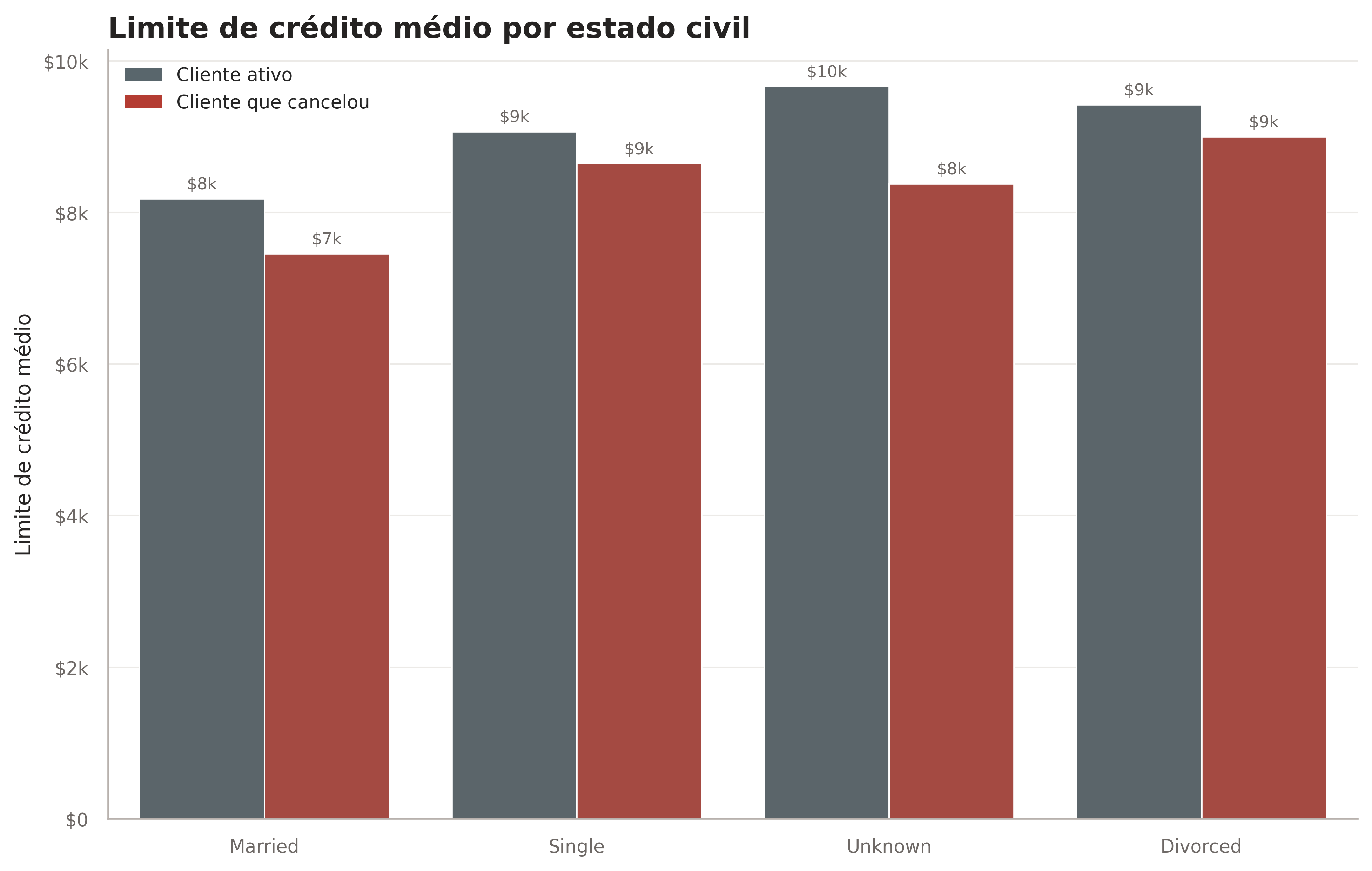
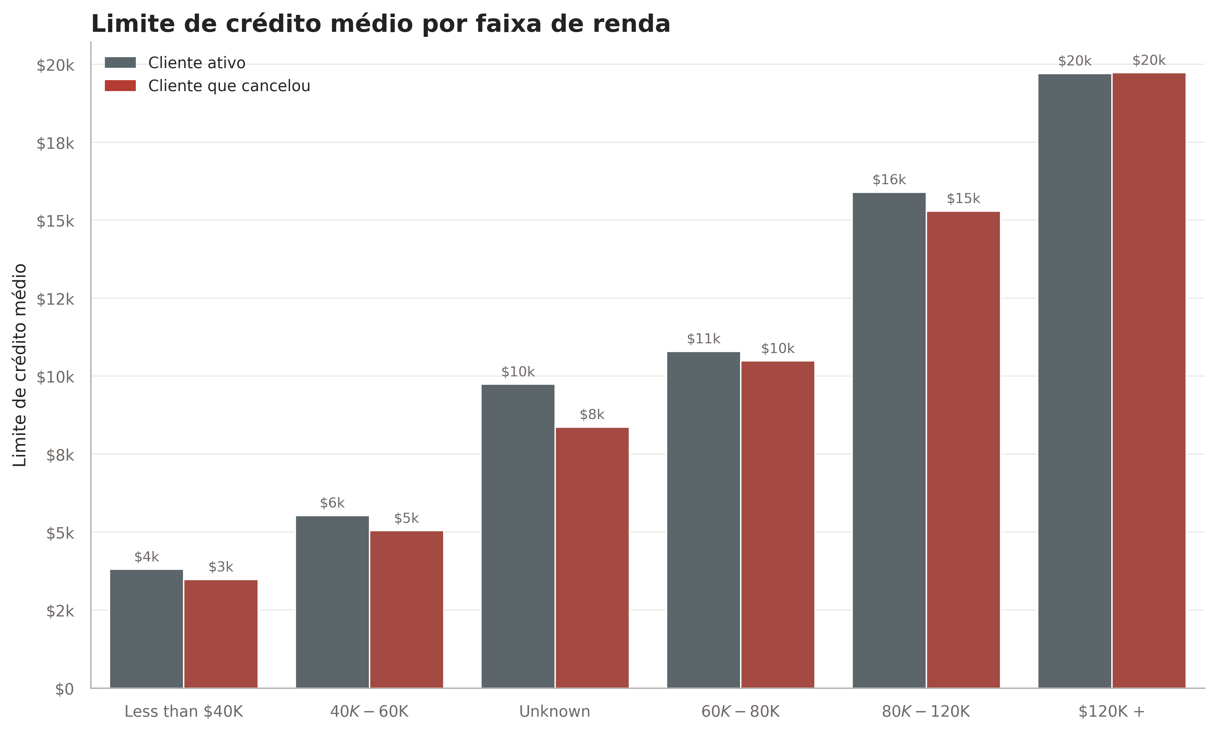
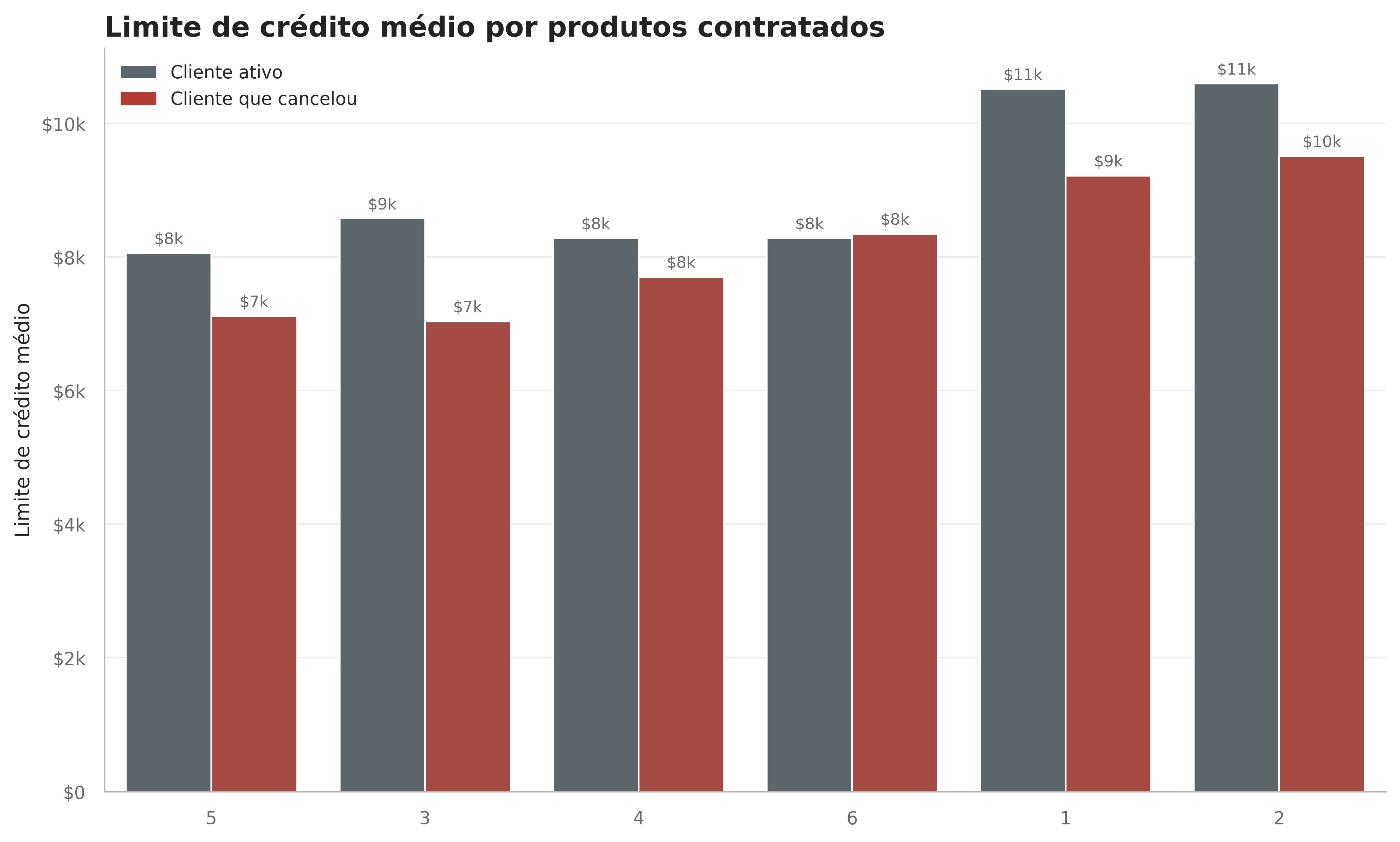
The code groups each of the selected categorical variables by the average credit limit, also including the churn variable to make the analysis easier when coloring the charts. To improve readability, I set an arbitrary limit for the y-axis based on the lowest value in each group, subtracting 2000 from the minimum for better display.
.png)
Dependents: As the number of dependents increases, the credit limit tends to grow.
Relationship: Customers without a partner generally have higher credit limits.
Average Income: The credit limit increases almost linearly with the customer's income.
Education: There is no apparent relationship between the customer's education level and their credit limit.
Products: The fewer products linked to the customer, the higher the credit limit tends to be.
Gender: Men have significantly higher credit limits than women.



3 - Correlation Matrix of Numerical Variables
This code selects only the numerical variables and builds a correlation matrix with pandas.corr(). Based on this matrix, a heatmap is plotted with Seaborn, where darker colors represent positive correlations and lighter colors indicate negative correlations.
.png)
Months As Customer vs Age: Strong correlation (0.79); older customers stay longer.
Credit Limit vs Average Open To Buy: Positive correlation (0.62); a higher limit means more available credit.
Total Transactions Amount vs Total Transactions Count: High correlation (0.81); more transactions produce a higher total amount.
Average Utilization Ratio vs Credit Limit: Negative correlation (-0.48); high limits reduce average utilization.
Average Open To Buy vs Average Utilization Ratio: Negative correlation (-0.54); more available credit reduces utilization.

4 - Share of Categories by Churn Likelihood
The code groups each of the selected categorical variables by the average credit limit, also including the churn variable to make the analysis easier when coloring the charts. To improve readability, I set an arbitrary limit for the y-axis based on the lowest value in each group, subtracting 2000 from the minimum for better display.
.png)
Relationship: Most customers are either single or married, with a small percentage divorced. Overall, being married lowers the likelihood of card churn.
Average Income: Customers with higher incomes are more prone to churn.
Education: People with higher education levels tend to be more likely to churn.
Overall Distribution: For income and education, the customer shares follow the expected pattern, in line with the natural distribution of these factors in the population.


5 - Customer Profile and Financial Variables
The code selects relevant financial columns, such as credit limit, total transaction amount and frequency of use, to explore how these factors relate to the customer profile, considering age and gender. To improve the visualization, we use a custom color palette that subtly distinguishes genders.
.png)
After age 30, women have a lower credit limit than men.
On the other hand, women use their credit card more than men.
The average transaction amount grows steadily until age 50, when it starts to decline.
Card utilization is stable across age groups, with men catching up to women around age 60.
The number of transactions stays constant until age 65, after which it starts to decline gradually.


6 - Card Type and Education Level
This code visually analyzes the distribution of education levels across card categories, using stacked histograms for each card type. Each chart uses a grayscale palette and organized legends, for a clear, comparative view.
.png)
The overwhelming majority of customers have a Blue card, showing how popular it is among users.
Education levels have no significant influence on the distribution of Blue, Silver and Gold cards.
Share at the Platinum Level: At the Platinum level, there is a considerable increase in the share of members with a Doctorate or Post-Doctorate, suggesting this card is more common among customers with advanced degrees.
Higher Education: Most customers have at least some higher education, which may reflect a more qualified customer profile, potentially more inclined to use premium credit cards.


7 - Statistical Distribution of Variables by Churn
This code creates a comprehensive view of the distribution of key churn-related variables, allowing visual comparisons between customers who canceled and those who stayed with the service. Each boxplot shows the median, the spread and the presence of outliers for the variables analyzed.
.png)
Customer loyalty to the bank ranges from 20 to 55 months, for both canceled and active customers.
Customers who canceled make considerably fewer transactions.
The outlier in the canceled group falls within the IQR of active customers, highlighting the difference in behavior.
Active customers make transactions with a higher average amount.
Despite the differences, credit limits are similar, with active customers having a slightly higher average.


PART 3
Data Preparation
1 - Strategies and Procedures
Just like cleaning a bedroom or a living room, cleaning a dataset requires a procedure: you can't start by sweeping and then throw the water on the floor! That is why, in this and other projects, I usually follow this order: removing useless columns, identifying and removing null values, identifying and removing outliers, creating dummy variables and encoding. This ensures a clean dataset, ready to work in an ML model.
2 - Handling Null Values
As I worked with the dataset, I noticed there were no "np.nan" values, the null values we usually work with, because they appeared in another form, as "Unknown". So I created a function to convert these into "np.nan", making the work easier. I then created two more functions: one that returned a dataframe with the sum of null values for each column, and another that generated a bar chart showing the percentage of missing values for each feature, that is, each column.
.png)

Looking at this chart, I saw that only a few rows had missing values. However, since the dataset has few rows, I did not want to drop any row with "np.nan". Instead, I chose to fill them with the value of the next cell, and to make this more accurate, I first sorted by "Credit_Limit", so neighboring cells would theoretically be closer to each other, since this column had already proven to be very impactful.
.png)
3 - Handling Outliers
To identify and remove outliers, I used John Tukey's well-known method, the same one used to build a boxplot. I created a function that returns a dataframe filtered between a lower and an upper bound, defined from the percentiles of the column being processed, selected the columns that could have outliers and applied the method to each of them.
.png)
4 - Encoding Categorical Variables
As a last step, I needed to encode the categorical variables as numbers. Since the dataset had relatively few rows, I tried to use "pd.get_dummies" as little as possible, because it creates extra columns for each category. So I only turned "Gender" and "Relationship_Status" into dummies, creating 3 new columns, since "drop_first = True".
.png)
For the other categorical variables, there was an implicit order of importance; for example, a "Platinum" card is expected to rank above a "Gold" card. I defined this order in several lists and used the sklearn.preprocessing function to assign numerical values that reflect this natural order. With the dataset completely clean, we move on to building the ML models.
PART 4
Machine Learning Predictions
1 - Initial Model Selection
First, I split the variables into "features" and "prediction", that is, "x" and "y", and used a StandardScaler so that differences in scale would not affect model training. Then I picked some of the main classic Machine Learning models to test their performance, such as DecisionTreeClassifier, RandomForest, XGBoost and others shown in the code. After running cross-validation to get reliable results, I got this:
.png)

Regardless of the model selected, the results are positive, with accuracy above 87% for every model. However, these models were created with default hyperparameters, which are probably not the best for maximizing accuracy. So I decided to tune 3 of them: XGBoost, because it is the most accurate model, and DecisionTreeClassifier and RandomForestClassifier, because their nature gives a clearer view of how the algorithm decides the "y" of a given row, especially the DecisionTreeClassifier. Let's tune:
2 - Tuning the DecisionTreeClassifier
Note that on this site I only show the tuning of one model, since the process is similar and it would not be interesting to say the same things 3 times in a row; if you are interested, the fully commented code for the others is on my GitHub. For the tuning, I used GridSearch with a parameter grid to run a 10-fold cross-validation. A simple calculation shows that about 50 thousand trees were trained and evaluated to find the best parameters and maximize accuracy, which proved to be well worth the effort:
.png)

Our decision tree went from 93.06% to 94.332% accuracy. That may seem like a small jump, but in business it can mean thousands or even millions of dollars more, depending on the size and reach of the company, so it is fair to say the tuning was a complete success!
3 - Comparing Predictions
Here are predictions on a test set the model had not seen yet, using the three previously optimized models, producing arrays with the results. The code then builds a dictionary to organize and compare these predictions with the actual values, which are the true labels of the test set. Finally, the dictionary is converted into a DataFrame to make it easier to see and analyze the differences.

As the cross-validation results suggested, the predictions are in line with reality, with few errors. In this specific slice, the only error occurs at index 3654, where the DTC and the RFC predicted a customer who would not cancel the card when, in reality, as the XGB predicted, it was a cancellation.
4 - Feature Importance Analysis
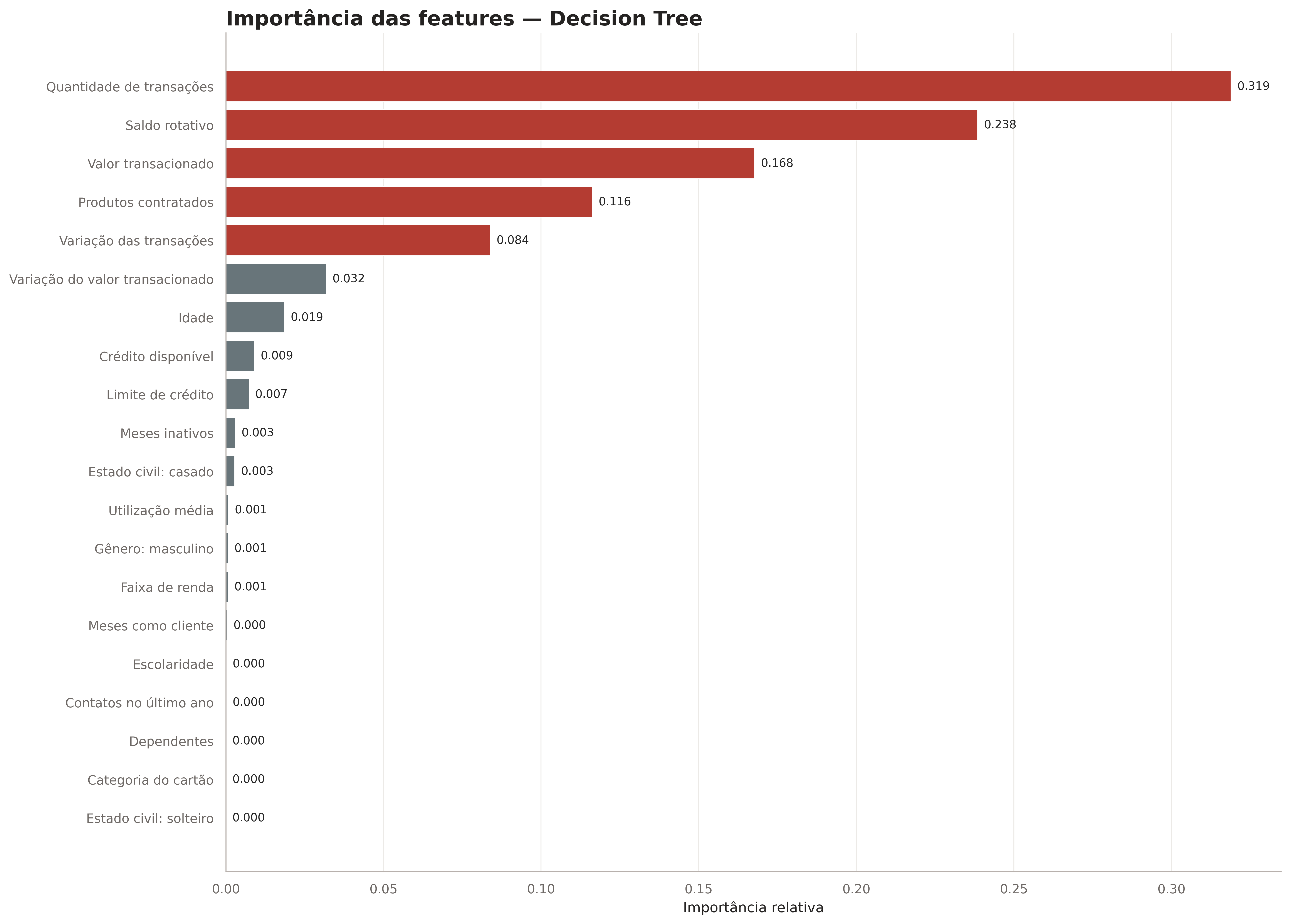
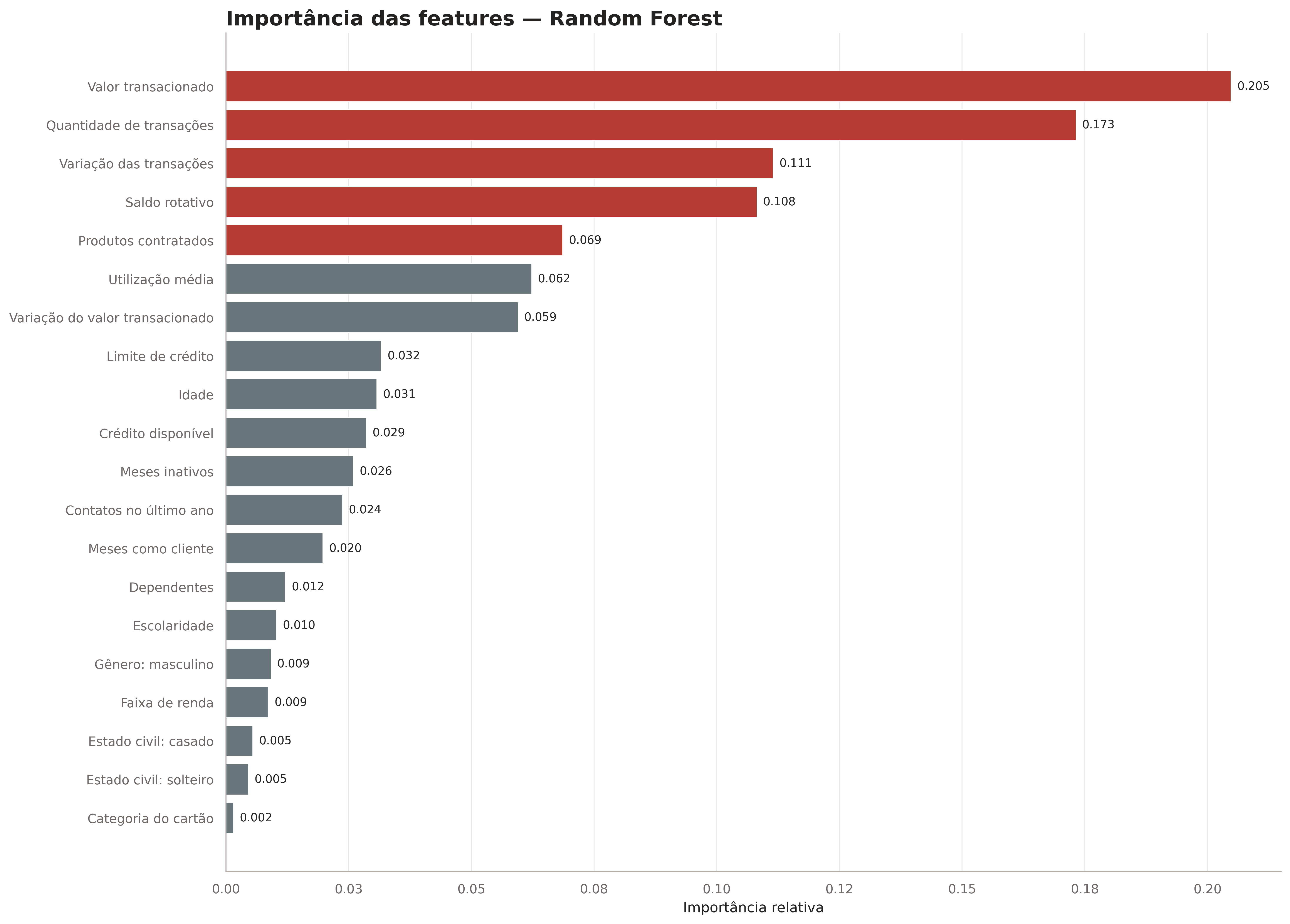
Using the feature_importances_ attribute, we can determine how important each column of the training dataset is, making it easier to identify the most relevant factors to consider. This analysis can better guide decision-making by the bank's staff. In the code, three horizontal bar plots are generated, using a combination of enumerate and zip to get the index and iterate over both lists at the same time.
.png)
These plots are interesting because they show how each model has its own way of understanding the information. Still, there are some clear patterns, such as columns like "Average Open to Buy" and "Income Lvl" always staying at the top, which indicates they are extremely relevant. On the other hand, others are consistently at the bottom, such as "Education", "Dependents" and "Gender", which shows these columns are almost dispensable for predicting customer churn and would probably not change training if removed.

4 - Confusion Matrix Analysis
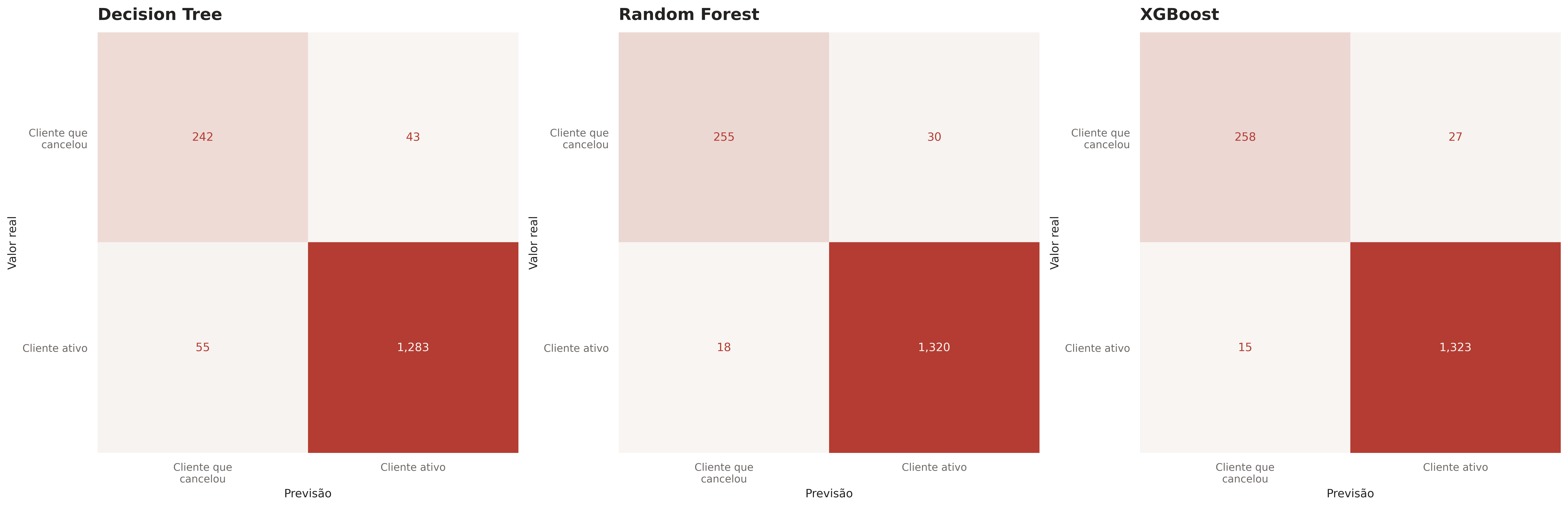
The confusion matrix is essential for evaluating classification models, since it gives a detailed view of true positives, false positives, true negatives and false negatives. This helps identify where the model makes mistakes and how to improve its accuracy. This code plots the confusion matrices for three classification models: XGBoost, Decision Tree and Random Forest. It calculates each matrix from the models' predictions and the true labels, shows them in subplots and displays each figure with the chosen palette and a custom title with the model name.
.png)
The matrices show similar results, as expected given the models' accuracy: the DecisionTreeClassifier has the most false positives and negatives, and XGBoost the fewest. This highlights the importance of small percentages mentioned above: even though XGBoost has only a few percentage points of accuracy advantage, it avoids false positives/negatives up to 2.5x better than the others. Assuming, as a low estimate, that a bank customer generates $100 in profit, this could mean up to $25,000 in extra profit.
5 - Visualizing the Decision Trees
The code visualizes the decision trees of three models: it uses Scikit-learn's "plot_tree" for the DTC and for a random estimator from the RFC, while XGBoost is visualized with its own function. The figure is set up with three subplots, and the charts show the tree structure up to three levels deep, with readable feature names. The full charts are available on GitHub.
.png)


6 - Insights and Conclusions
Finally, after a detailed analysis, we gathered a wide range of valuable insights. They are more than enough to give complete, well-founded answers to the questions raised at the start of the project, and here are the answers:
What is the profile of the customers most likely to cancel their card?
Older customers who make fewer transactions and have credit limits similar to active customers are at higher risk of canceling.
How does customer gender affect financial condition and cancellation rates?
Women tend to have lower credit limits but use their cards more often. This leads to different usage patterns between genders.
Does education level influence the likelihood of canceling the card?
People with higher education levels tend to be more likely to cancel their cards
Do customers who use their card more receive higher or lower credit limits?
Customers who make more transactions often receive higher credit limits, since total transaction amount is directly related to the limit.
Are customers with high incomes more likely to cancel their cards?
Customers with higher incomes show a greater tendency to cancel.
What behaviors are common among customers who cancel their cards?
Customers who cancel tend to make fewer transactions and use their card less actively than those who stay with the service.
We also met the requirements for the Machine Learning models, building three models with accuracy above 85%. Each model comes with a detailed analysis of feature importance, which clearly and effectively identifies the main factors driving the predictions.
In addition, the DecisionTreeClassifier meets the high interpretability requirement, standing out for its simple structure, which allows easy visualization and clear, direct decision rules using a single tree. This is unlike more complex models such as RandomForestClassifier and XGBoost, which use multiple decision trees (Random Forest) or a set of trees with adaptive learning (XGBoost).